Aggregations

Custom Column Aggregations are used to set or change the summation logic used on columns presented in the data model. By creating or 'changing' the aggregation type of a metric or hierarchy column, the engine effectively adds a new virtual column to the data model that represents a new way to quantify query results.

Custom Columns, by definition are executed at the grain, and so these columns (usually) produce different results compared to changing the semantic operations on existing columns - which is desirable depending on the business or analytic problem being resolved.

Note: Custom Columns allow the user to add granular logic to an existing model. This functionality is not available on MS OLAP, Tabular and SAP BW cubes and models since this is not possible on a predefined model framework.

Custom Column Aggregation Types

Aggregation options vary depending on the data type of the raw data columns.

Numeric Custom Columns

The aggregations for numeric data type columns can be set to count, distinct count, minimum, maximum, sum, average, variance (both sample and population), standard deviation (both sample and population), first quartile (25th percentile), median (50th percentile) and third quartile (75th percentile).

The grid below is based on the sample In-memory database.

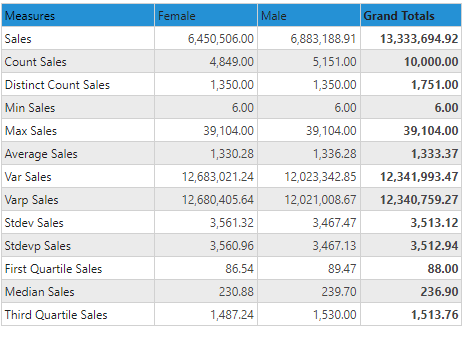
The sales column is a numeric column on the transaction fact table. Its usual aggregation is a simple, additive summation. From the preceding table we can see:

• Summing every row of the sales numbers produces a value of 13.33M
• Counting the rows produces a value of 10,000 - which is the number of actual rows in the fact table itself.
• Distinct count (unlike count) counts the number of distinct sale numbers that appear across the entire table - which is 1751 unique values.
• Minimum sales measures the row with the lowest number in the table - "6"
• Maximum sales measures the row with the highest number in the table - "39104"
• Average sales is simply the total sum, divided by the number of rows 1,333 (13.33M/10000)
• Variance sales (based on sample math) is the statistical variance using all the individual sales numbers in the column
• Variance "P" sales (based on population math) is the statistical variance using all the individual sales numbers in the column
• Standard Deviation (based on sample math) is the statistical standard deviation found across all the individual sales numbers in the column
• Standard Deviation "P" (based on population math) is the statistical standard deviation found across all the individual sales numbers in the column
• First quartile sales shows the single sales row that is found at the 25th percentile. In this specific case its on row 2,500.
• Median sales shows the single sales row that is found at the 50th percentile - or the middle. In this specific case its on row 5,000.
• Third quartile sales shows the single sales row that is found at the 75th percentile. In this specific case its on row 7,500.

Notice, that when the aggregation is additive, the split between male and female can be easily added up to the total (sum, count). While for all other non-additive aggregations, they cannot because the logic produces different results based on the sub-sets of female rows and male rows (first quartile sales for males plus first quartile sales for females does not match first quartile sales across the entire dataset).

Generally, additive aggregation logic can be solved in both granular and semantic calculations while non-additive aggregation logic can only be solved by changing the functional operations on the grain. This is why changing granular aggregation logic is a pivotal capability in analytics.

Non-numeric Custom Columns

Aggregation

The aggregations for non-numeric data type columns can be set to count, distinct count, minimum and maximum only.

The transaction ID column is a text based ID column on the transaction fact table. It is usually not aggregated. From the preceding table we can see:

• Counting the rows produces a value of 10,000 - which is the number of actual rows in the fact table itself. This matches the same count as the sales count above since we are counting the exact same number of rows in the same table.
• Distinct count (unlike count) counts the number of distinct transaction IDs that appear across the entire table - which is 9955 unique values.(technically if they were truly unique it should have been 10,000).
• Minimum transaction ID is the lowest alphanumeric value in the column- "0017DB....."
• Maximum transaction ID is the highest alphanumeric value in the column- "FFF04D....."

Notice the that split between male and female do add up for the transactional aggregations because male and female values are stamped on the fact table as well and there are 10,000 unique transactions ID's through the table.

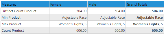
The product column is a text based column on the product dimension table. It is usually not aggregated. From the preceding table we can see:

• Counting the rows produces a value of 606 - which is the number of actual rows in the product table itself.
• Distinct count (unlike count) counts the number of distinct products that appear across the entire table - which is 504 unique values.
• Minimum product is the lowest alphanumeric value in the column- "Adjustable Race"
• Maximum product is the highest alphanumeric value in the column- "Women's Tights"

Notice the that split between male and female do NOT add up, because they are unrelated to this table (there is no direct nexus to the product table inferred from the gender table via the fact table unless bi-directional filtering is enabled).

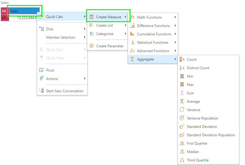
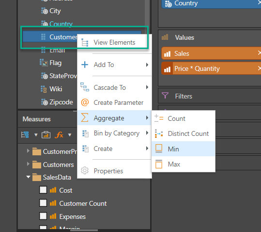
Adding Custom Column Aggregations

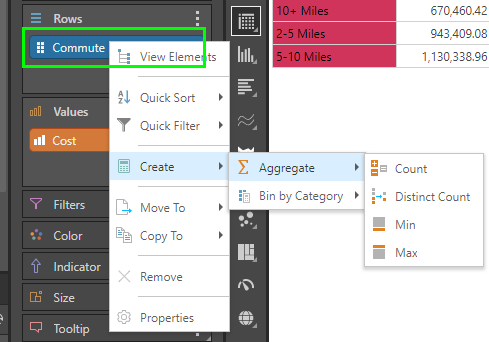
Aggregations can be added from the hierarchy and /or measure element trees.

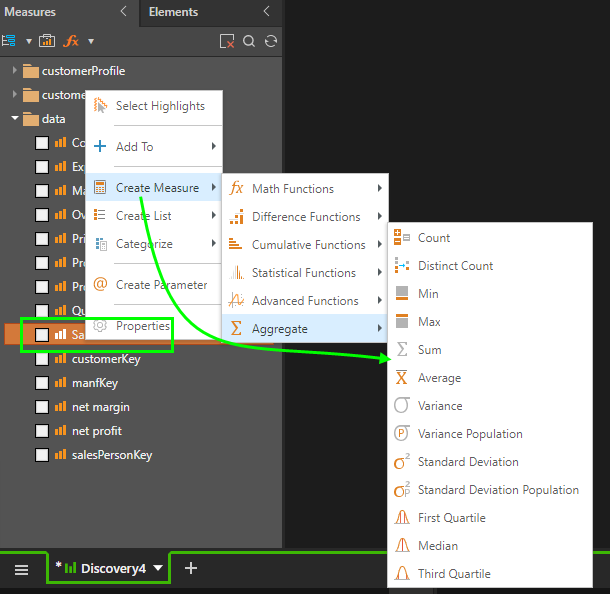
Aggregations and string functions can also be added from the drop zones.

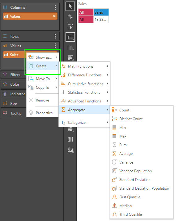
Aggregations for values can also be done directly off visuals. This is not possible for hierarchies though.